

NRTL activity coefficients for ethanol–water: a worked example
How far does an equimolar ethanol–water liquid at 343.15 K depart from an ideal solution? Follow one live ChETL calculation from the Library parameters to τ, G, ln γ and γ.
- Mixture
- Ethanol (1) / water (2)
- Temperature
- 343.15 K (70 °C)
- Liquid composition
- x₁ = x₂ = 0.5
- Model
- NRTL · Library parameters
- Ethanol
- γ₁ = 1.2449
- Water
- γ₂ = 1.4739
Each species in this liquid has a higher escaping tendency than it would in an ideal solution of the same composition. These are model predictions from the stated parameters, independently reproduced; they are not a comparison with experimental data.
Fix the mixture, its order and the state.
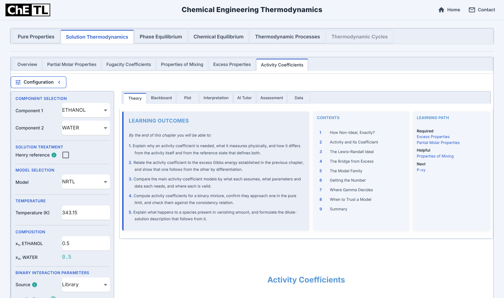
Open Solution Thermodynamics → Activity Coefficients. The topic opens on ETHANOL/WATER, NRTL and Library parameters at 323.15 K and x₁ = 0.4; change only the temperature and composition.
Choose the mixture, model and state
Component 1 is ETHANOL and component 2 is WATER; that order fixes every subscript below. Henry reference stays unchecked, so both species use the pure-liquid (Lewis–Randall) reference. The model is NRTL with Library parameters; set T = 343.15 K and x₁ = 0.5, then Calculate.
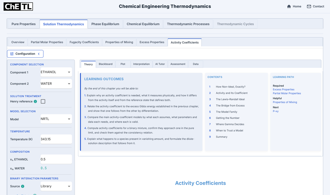
Configuration: components, treatment, model, temperature and composition. Inspect the resolved directional coefficients
Expanding Coefficients shows the Library set already ordered for ethanol(1)–water(2), with its valid temperature range. The narrow b fields truncate the displayed digits (284.2856 and −636.726 K); the Blackboard Knowns show the full values.
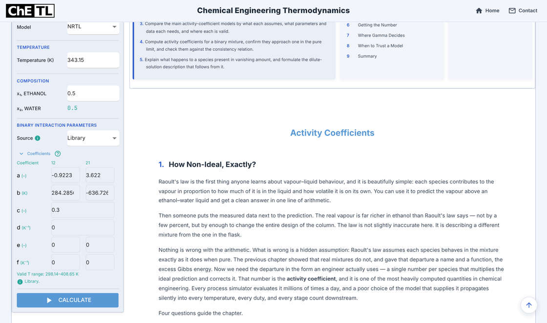
Configuration: Library coefficients a–f and valid range.
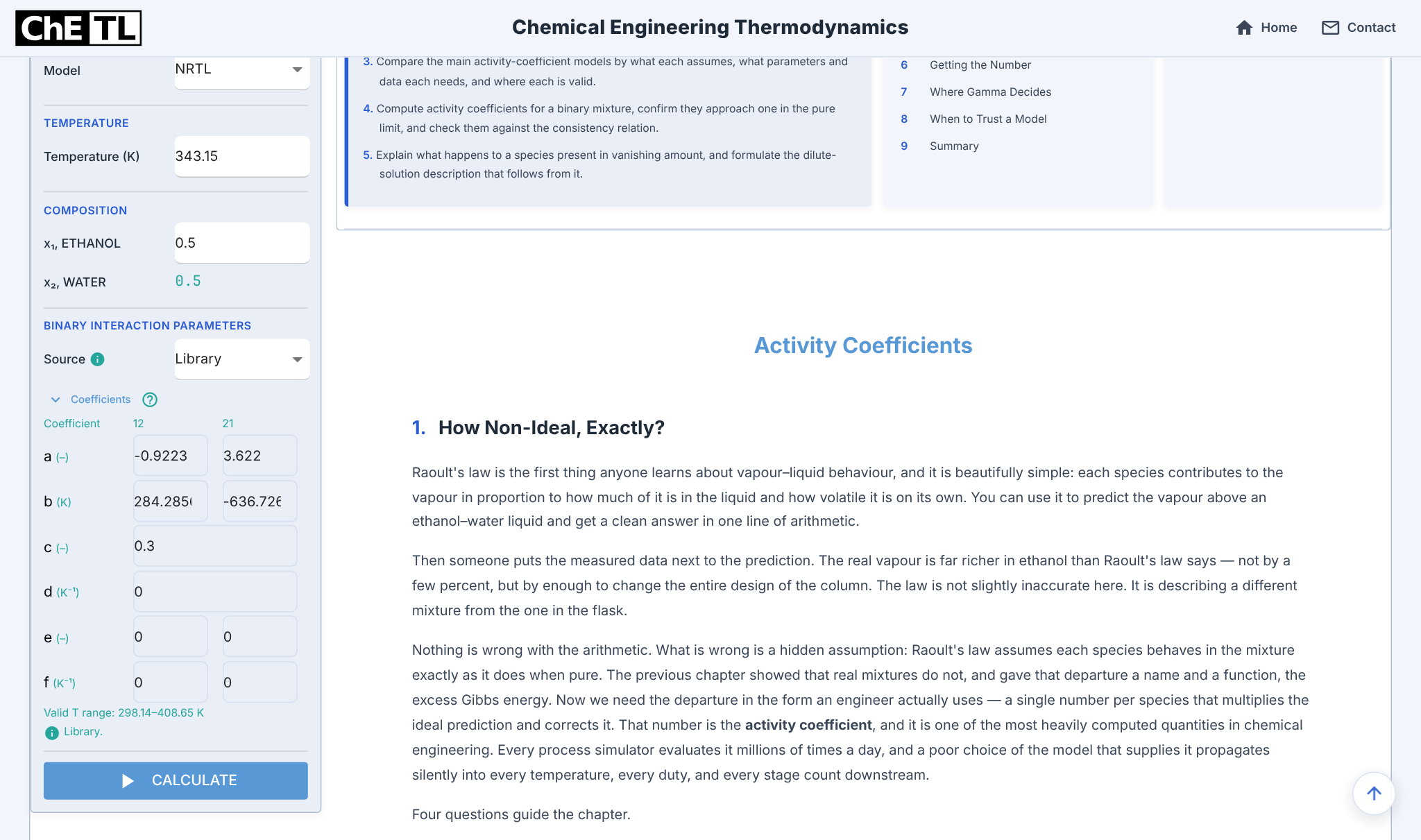
The known quantities are temperature, composition and the model parameters. The unknowns are γ₁ and γ₂. Pressure is not an input: this NRTL form has no pressure dependence, a usual approximation for liquids at moderate pressure.
Compare the mixture with its pure liquids.
The Theory tab defines activity against a stated reference; its strategy places NRTL among the routes to γ.
Activity and its coefficient
The Theory chapter defines the activity against a stated standard state and the activity coefficient as its ratio to mole fraction.
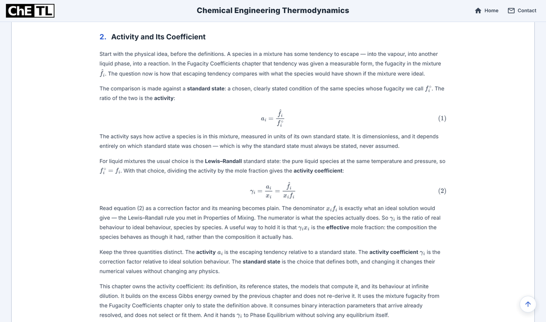
Theory tab: activity, standard state and activity coefficient. Choose a route to γ
The solution strategy separates ideal, fitted-model and predictive routes. A fitted model such as NRTL first needs resolved parameters with their provenance.
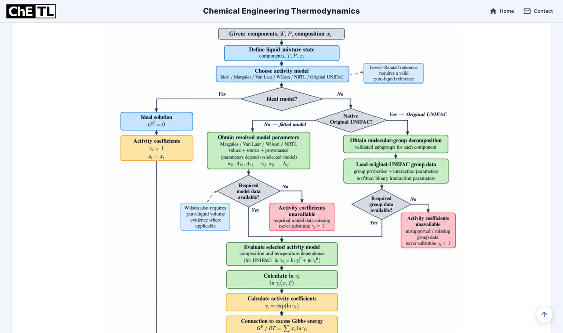
Solution strategy, upper part (view 1 of 2). Evaluate, then check
The model is evaluated at the configured temperature and composition, followed by exponentiation, the excess-Gibbs-energy link and pure-limit and Gibbs–Duhem checks.
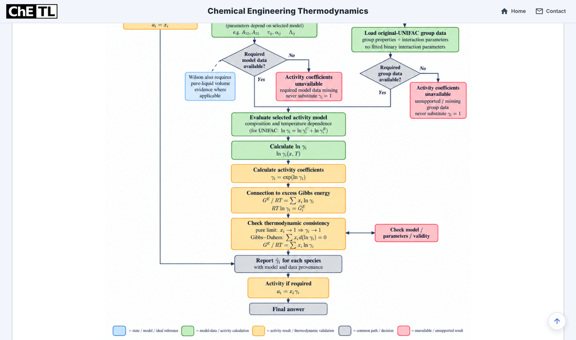
Solution strategy, lower part (view 2 of 2; the views overlap).
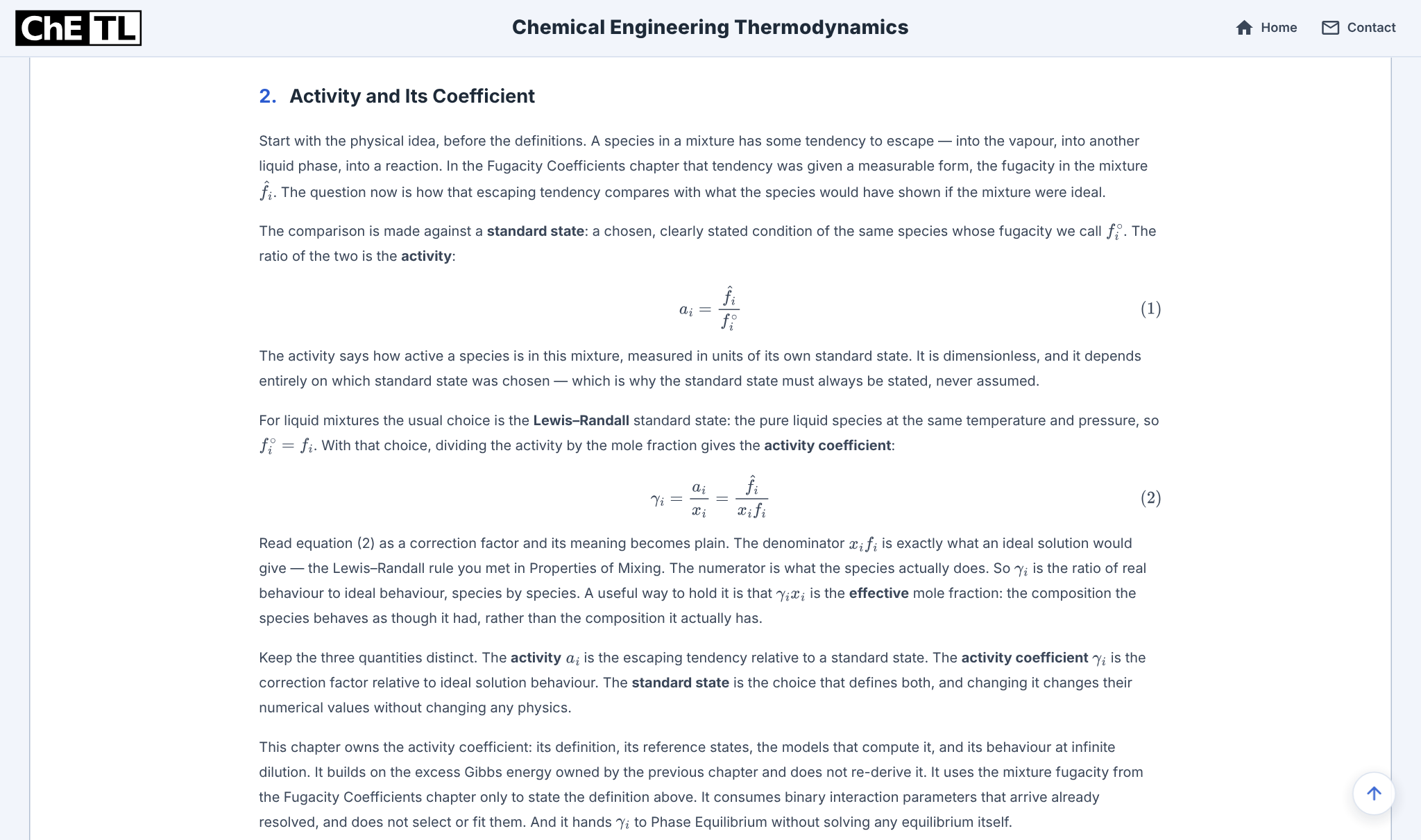
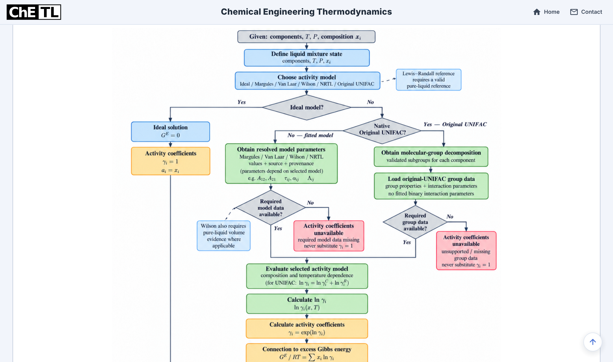
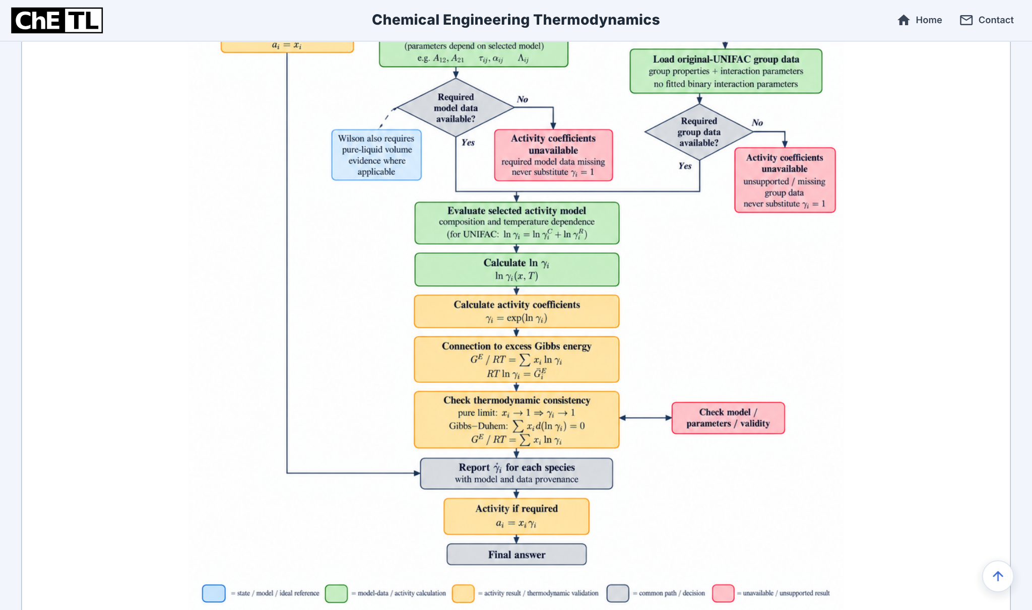
Reference state, activity and activity coefficient
For each species the reference is its pure liquid at the same temperature and pressure (Lewis–Randall), so the standard-state fugacity is fi° = fi. The activity compares the species’ fugacity in the mixture with that reference; the activity coefficient compares the activity with the mole fraction:
ai = f̂i / fi°, γi = ai / xi = f̂i / (xifi)
The activity is an effective mole fraction; γ is the correction factor. Here a₁ = x₁γ₁ = 0.6225 and a₂ = 0.7369, compared with 0.5 for an ideal solution. With this reference, γi → 1 as xi → 1 for every model.
ln γi = ḠiE / (RT)
The logarithm of each activity coefficient is the corresponding partial molar excess Gibbs energy divided by RT. The molar excess Gibbs energy therefore satisfies
GE / (RT) = Σi xi ln γi
NRTL at the configured temperature
τ12 = a12 + b12/T + e12 ln T + f12T, τ21 likewise, α = c + d(T − 273.15)
G12 = exp(−ατ12), G21 = exp(−ατ21)
ln γ1 = x22 [ τ21 (G21 / (x1 + x2G21))2 + τ12G12 / (x2 + x1G12)2 ]
ln γ2 = x12 [ τ12 (G12 / (x2 + x1G12))2 + τ21G21 / (x1 + x2G21)2 ]
The Library stores this pair as water–ethanol. Using ethanol as component 1 exchanges every directional term (a12↔a21, b, e, f); α is shared. Keeping the source order by mistake would exchange τ12 and τ21 and give different coefficients for each species.
| Term | a / – | b / K | e / – | f / K⁻¹ | τ at 343.15 K | RTτ / J mol⁻¹ |
|---|---|---|---|---|---|---|
| τ12 | −0.9223 | 284.2856 | 0 | 0 | −0.09384 | −267.7 |
| τ21 | 3.622 | −636.726 | 0 | 0 | 1.7665 | 5039.9 |
α = c + d(T − 273.15) with c = 0.3 and d = 0 K⁻¹. The a–f values are temperature-correlation coefficients: b has units of kelvin and τ is dimensionless. They are not interaction energies. The energy parameter the correlation implies is gij − gjj = RTτij (last column, R = 8.314462618 J mol⁻¹ K⁻¹). Enter a source’s parameters only in the form its correlation defines.
Read the actual Blackboard trace.
Four successive views show the whole trace; each starts where the last left off. The substitutions come from the running platform.
Problem, knowns and assumptions
The trace records the composition, temperature, the three NRTL coefficient groups from the Library, their valid range and the Lewis–Randall reference. It assumes a single liquid phase at the stated temperature.
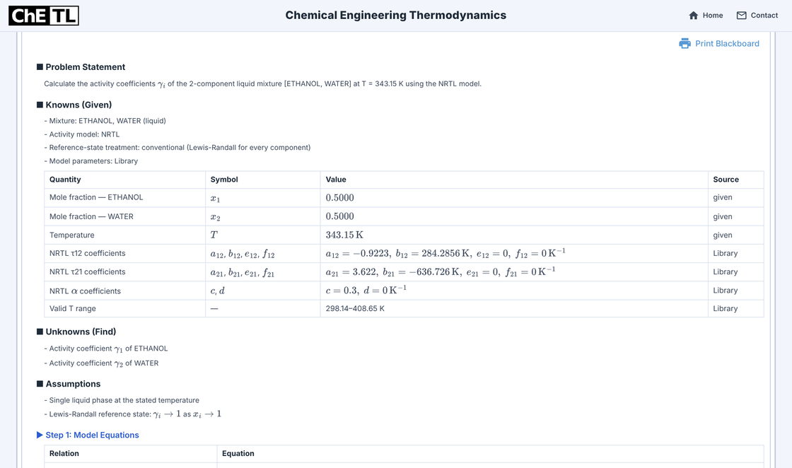
Blackboard: problem, knowns, unknowns and assumptions. The model equations
Step 1 lists the definition of γ, the τ and α correlations, the NRTL G factors and the two binary ln γ relations before any substitution.
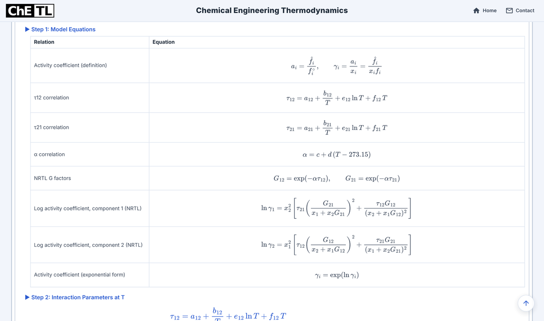
Blackboard: Step 1 model equations. Evaluate τ, α and the G factors
At 343.15 K, τ₁₂ = −0.09384 and τ₂₁ = 1.7665, with α = 0.3. Then G₁₂ = 1.0286 and G₂₁ = 0.5886.
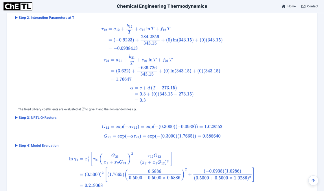
Blackboard: Steps 2–4, τ and α at T, G factors, ln γ₁. Activity coefficients
ln γ₁ = 0.2191 and ln γ₂ = 0.3879, so γ₁ = 1.2449 for ethanol and γ₂ = 1.4739 for water.
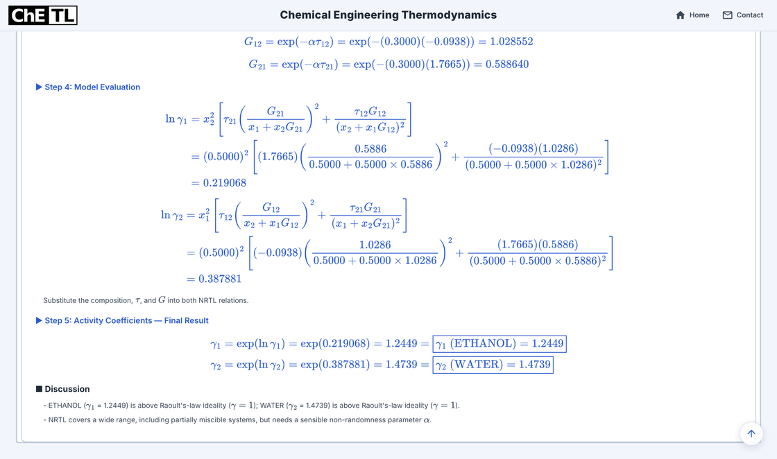
Blackboard: Steps 4–5, ln γ and γ for both species.
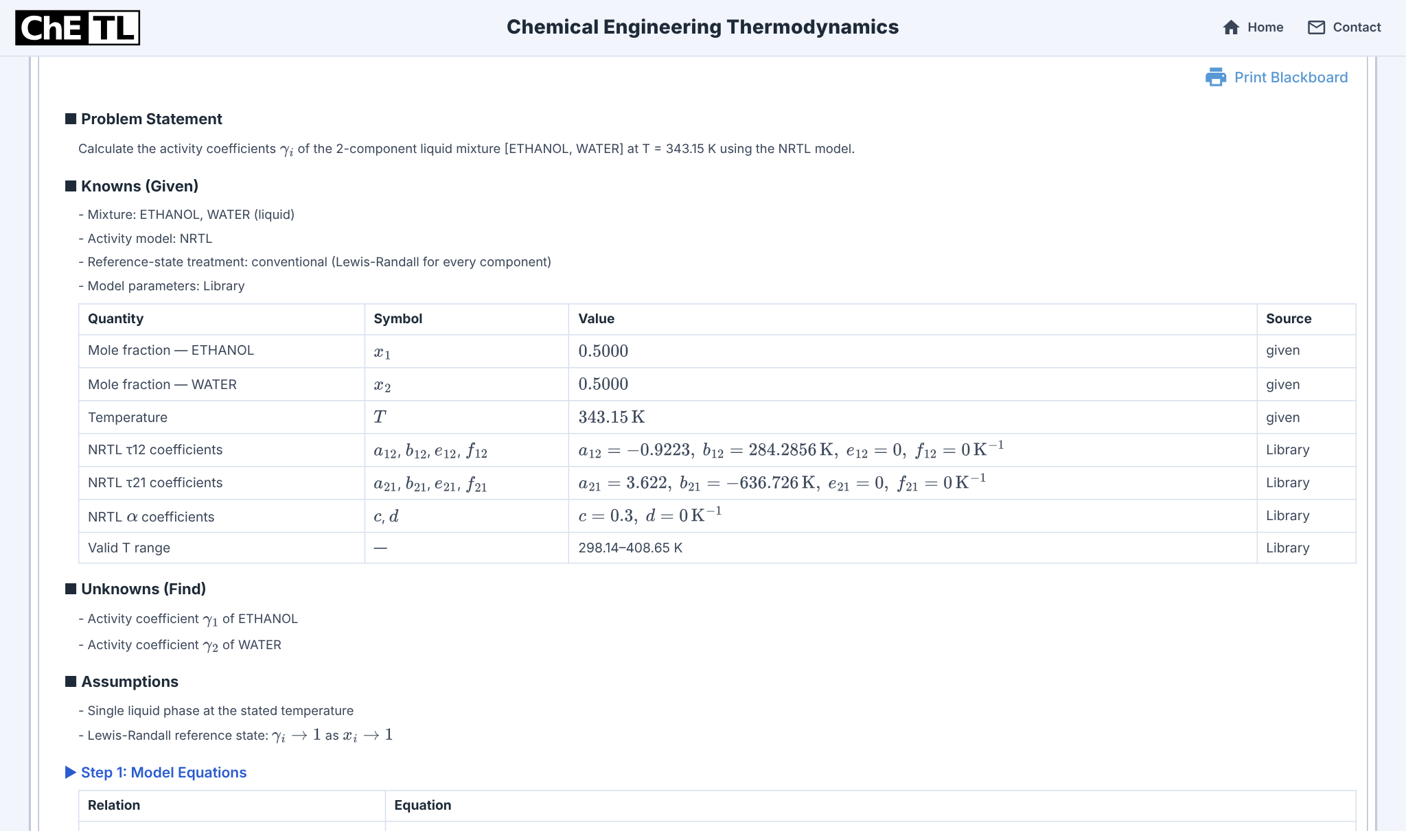
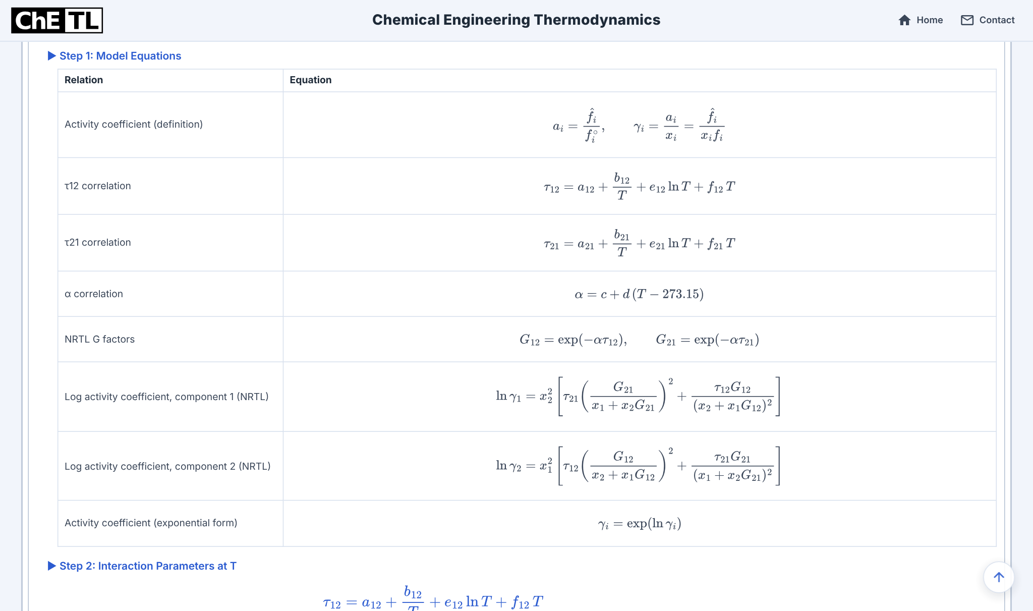
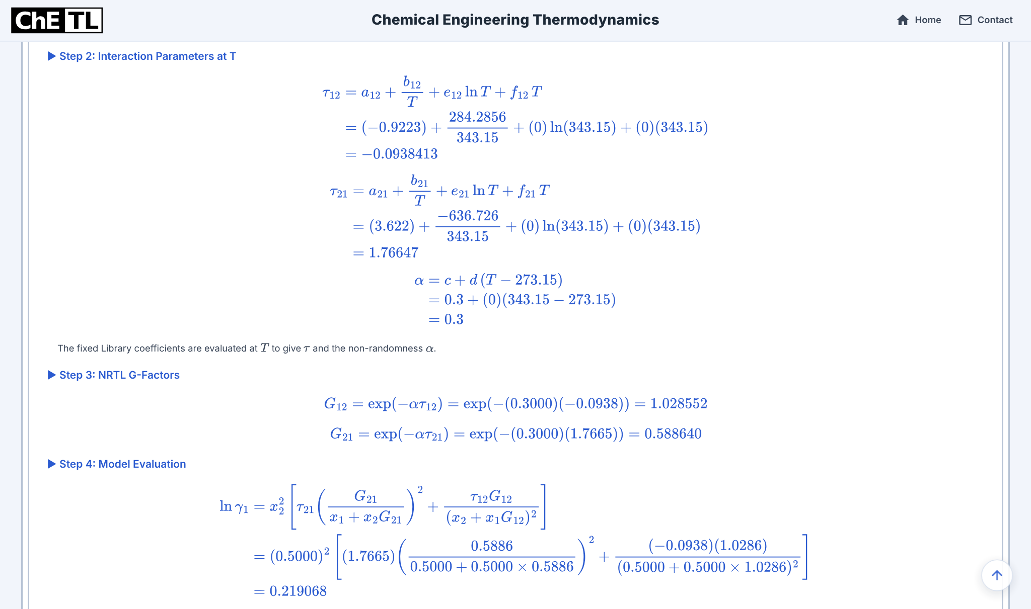
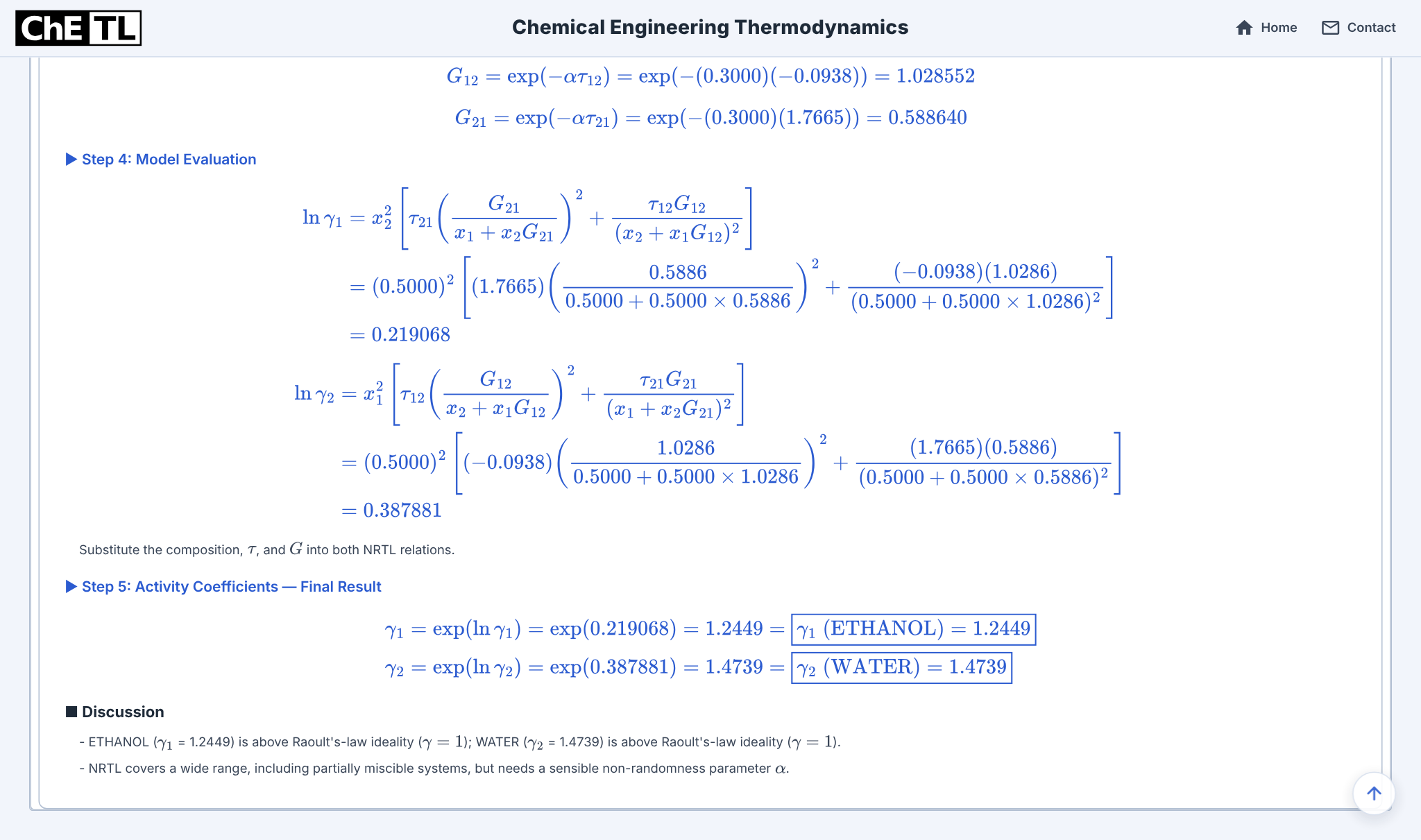
The Blackboard displays 343.15 K. Intermediate values are displayed rounded, so recomputing from them can differ in the last digit.
See how γ changes with composition.
The Plot tab sweeps ln γ₁ and ln γ₂ across the composition range at the configured temperature and marks the configured state.
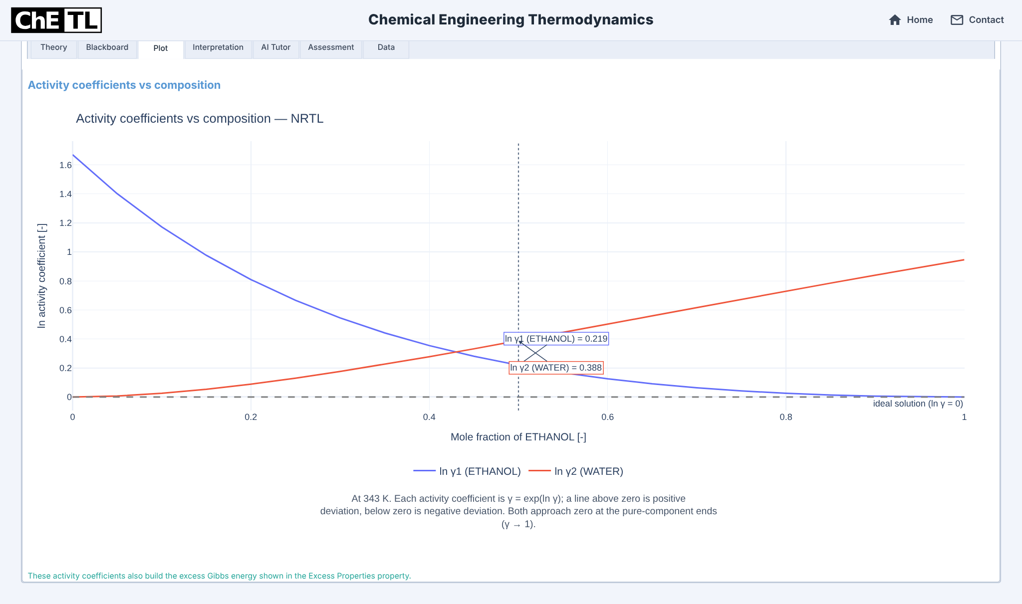
Each curve reaches zero at its own pure-component end: ln γ₁ = 0 at x₁ = 1 and ln γ₂ = 0 at x₁ = 0, as the pure-liquid reference requires. At the opposite ends are the infinite-dilution limits, ln γ₁∞ = τ₂₁ + τ₁₂G₁₂ = 1.670 (γ₁∞ = 5.31) and ln γ₂∞ = τ₁₂ + τ₂₁G₂₁ = 0.946 (γ₂∞ = 2.58). One curve falls while the other rises, as the Gibbs–Duhem relation Σxi d ln γi = 0 requires at constant T and P.
Explain the deviation, and stop at what γ shows.
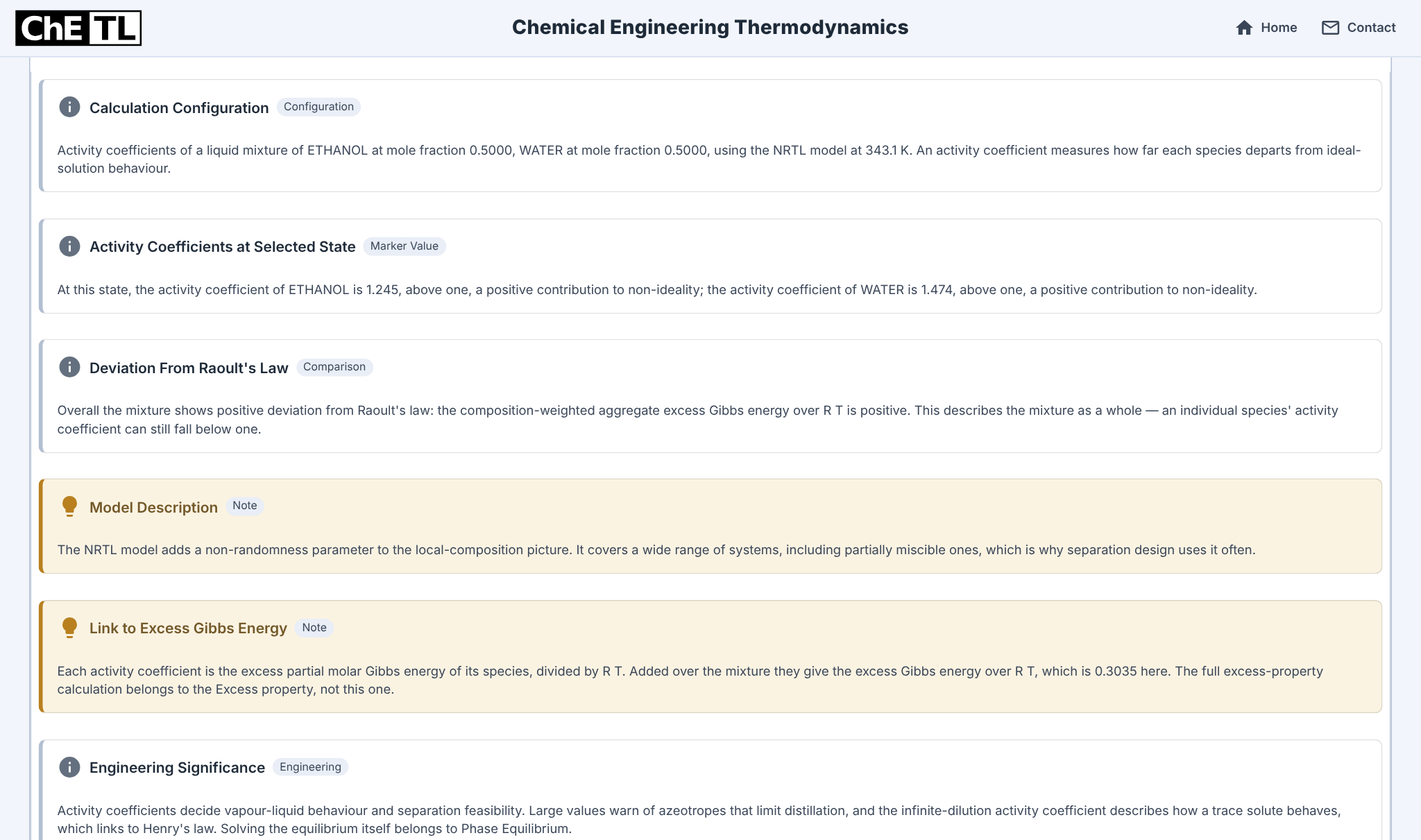
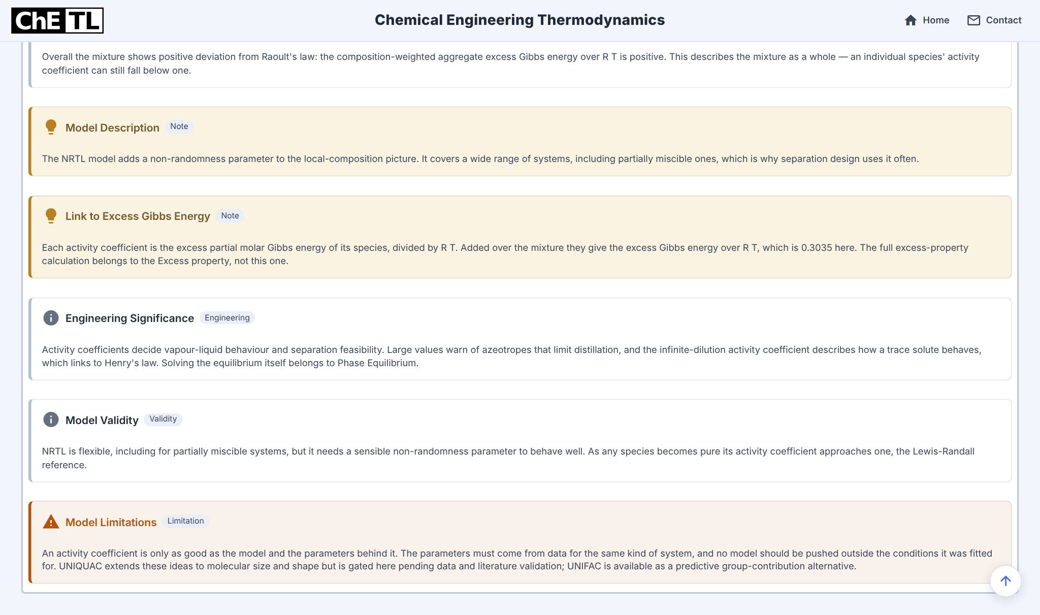
Two successive views show every Interpretation card.
Both species escape more readily than ideal
Both coefficients exceed one, and GE/RT = Σxi ln γi = 0.3035 is positive: a positive deviation from Raoult’s law at this composition. The configuration card rounds the temperature to 343.1 K; the input is 343.15 K.
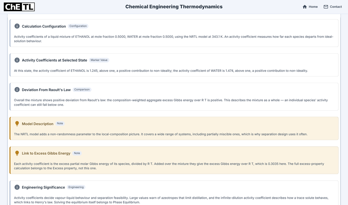
Interpretation: state, deviation, model and the excess-Gibbs-energy link. What γ alone does not decide
The remaining cards place the result in context and state its limits. Their remark that large values can warn of azeotropes is general guidance: an azeotrope also depends on the pure-component vapour pressures, so it needs a phase-equilibrium calculation.
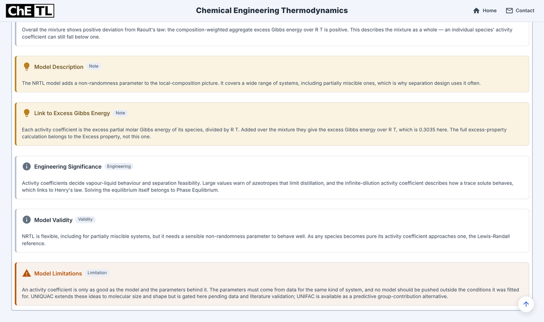
Interpretation: significance, validity and limitations.
Where these coefficients are used. In modified Raoult’s law, yiP = xiγiPisat. The ethanol–water P–xy worked example uses these same γ values at this state, with saturation pressures, to find the bubble pressure and first-vapour composition.
Take the composition data with you.
The Data tab holds the 21 plotted states, with copy, CSV and Excel export controls.
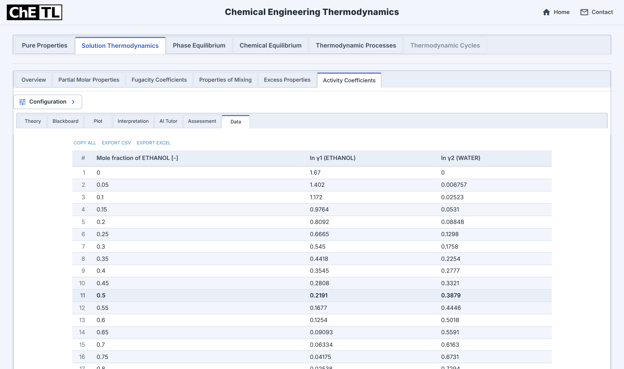
Inspect the plotted values
| x1 | ln γ1 | ln γ2 |
|---|---|---|
| 0.00 | 1.6699 | 0.0000 |
| 0.05 | 1.4015 | 0.0068 |
| 0.10 | 1.1723 | 0.0252 |
| 0.15 | 0.9764 | 0.0531 |
| 0.20 | 0.8092 | 0.0885 |
| 0.25 | 0.6665 | 0.1298 |
| 0.30 | 0.5450 | 0.1758 |
| 0.35 | 0.4418 | 0.2254 |
| 0.40 | 0.3545 | 0.2777 |
| 0.45 | 0.2808 | 0.3321 |
| 0.50 | 0.2191 | 0.3879 |
| 0.55 | 0.1677 | 0.4446 |
| 0.60 | 0.1254 | 0.5018 |
| 0.65 | 0.0909 | 0.5591 |
| 0.70 | 0.0633 | 0.6163 |
| 0.75 | 0.0417 | 0.6731 |
| 0.80 | 0.0254 | 0.7294 |
| 0.85 | 0.0136 | 0.7850 |
| 0.90 | 0.0057 | 0.8396 |
| 0.95 | 0.0014 | 0.8933 |
| 1.00 | 0.0000 | 0.9460 |
Assumptions and limits
- One liquid phase at the stated temperature; the calculation does not test liquid–liquid stability. γ > 1 alone does not show that a second liquid phase forms.
- γ alone does not show an azeotrope. That needs the vapour pressures as well, as in the P–xy example.
- The Library coefficients are used inside their stated 298.14–408.65 K range. A correct evaluation shows that the equations were satisfied, not that NRTL with these parameters matches experimental data for this mixture.
- Activity coefficients depend on the chosen reference state. A Henry-reference (dilute-solute) treatment would report different numbers for the same mixture.
Check your understanding
Show the answer and explanations
- Correct. The activity is a1 = x1γ1 = 0.5 × 1.2449 = 0.6225, measured against the pure-liquid reference. γ1 is the factor between activity and mole fraction.
- Not supported. An azeotrope depends on γ and the pure-component vapour pressures. The P–xy example combines both; γ alone cannot decide it.
- Not supported. Phase splitting needs a stability test on the Gibbs energy of mixing over composition. This calculation assumes one liquid phase and does not perform that test.
- Not supported. γ1 depends on composition: it approaches 1 as x1 → 1 and 5.31 at infinite dilution.
Sources and review
Unannotated snapshots were captured on 10 November 2026 from a local run of the current ChETL source with the settings shown in Set up. Each is a complete 1366 × 808 px viewport at one fixed scale, including the platform header; nothing was cropped, retouched or edited.
A separate Python calculation, written without the platform’s code, reproduces τ, α, G, ln γ and γ at the selected state and all 21 plotted points from the source coefficients. It also checks ln γ against a numerical derivative of nGE/RT, the pure-component limits and the Gibbs–Duhem relation. This AI-assisted check establishes numerical consistency, not experimental validation or human peer review.
Model reference: Renon and Prausnitz, AIChE Journal 14 (1968) 135; Smith, Van Ness, Abbott and Swihart, Introduction to Chemical Engineering Thermodynamics, 9th ed. Parameters: ChETL Library, recovered APV150 VLE-RK databank record. Editorial responsibility rests with the ChETL Scientific Editor.
To try the case, sign in and enter the settings in Set up. Then change the composition or temperature, or switch to another activity model, and compare. Continue with the Solution Thermodynamics guide or the P–xy worked example.
Corrections: info@chetl.org.